Binary Stochastic Neurons
This post is a rebroadcast of R2RT’s bst post. It talks about ST and REINFORCE estimator used in BSN network.
import numpy as np
import tensorflow as tf
from tensorflow.examples.tutorials.mnist import input_data
import matplotlib.pyplot as plt
mnist = input_data.read_data_sets('MNIST_data/', one_hot=True)
from tensorflow.python.framework import ops
from enum import Enum
import seaborn as sns
sns.set(color_codes=True)
def reset_graph():
    if 'sess' in globals() and sess:
        sess.close()
    tf.reset_default_graph()

def layer_linear(inputs, shape, scope='linear_layer'):
    with tf.variable_scope(scope):
        w = tf.get_variable('w', shape)
        b = tf.get_variable('b', shape[-1:])
    return tf.matmul(inputs, w) + b

def layer_softmax(inputs, shape, scope='softmax_layer'):
    with tf.variable_scope(scope):
        w = tf.get_variable('w', shape)
        b = tf.get_variable('b', shape[-1:])
    return tf.nn.softmax(tf.matmul(inputs, w) + b)

def accuracy(y, pred):
    correct = tf.equal(tf.argmax(y,1), tf.argmax(pred,1))
    return tf.reduce_mean(tf.cast(correct,tf.float32))

def plot_n(data_and_labels, lower_y = 0., title="Learning Curves"):
    fig, ax = plt.subplots()
    for data, label in data_and_labels:
        ax.plot(range(0,len(data)*100,100),data, label=label)
    ax.set_xlabel('Training steps')
    ax.set_ylabel('Accuracy')
    ax.set_ylim([lower_y,1])
    ax.set_title(title)
    ax.legend(loc=4)
    plt.show()

class StochasticGradientEstimator(Enum):
    ST = 0
    REINFORCE = 1
Binary stochastic neuron with straight through estimator
def binaryRound(x):
    """
    ROunds a tensor whose values are in [0,1] to a tensor with values in {0, 1},
    using the straight through estimator for gradient.
    """

    g = tf.get_default_graph()

    with ops.name_scope("BinaryRound") as name:
        with g.gradient_override_map({"Round": "Identity"}):
            return tf.round(x, name=name)
## I'm bit confused here as well. Not sure about if BernoulliSample_ST is implemented correctly.
def bernoulliSample(x):
    """
    Uses a tensor whose values are in [0, 1] to sample a tensor with values in {0,1}.

    E.g.,:
    if x is 0.6, bernoulliSample(x) will be 1 with probability 0.6, and 0 otherwise.
    and the gradient will be pass-through(identity). Note gradient for (x-tf.random_uniform) is still preserved
    """

    g = tf.get_default_graph()

    with ops.name_scope("BernoulliSample") as name:
        with g.gradient_override_map({"Ceil": "Identity", "Sub": "BernoulliSample_ST"}):
            return tf.ceil(x - tf.random_uniform(tf.shape(x)),name=name)

@ops.RegisterGradient("BernoulliSample_ST")
def bernoulliSample_ST(op, grad):
    # the grad is the op'output w.r.t output (x-tf.random_uniform), seems to be 1 to me??
    return [grad, tf.zeros(tf.shape(op.inputs[1]))]
Combine passthrough with bernoulliSample we then have bsn
def passThroughSigmoid(x, slope=1):
    """Sigmoid that uses identity function as its gradient"""
    g = tf.get_default_graph()
    with ops.name_scope("PassThroughSigmoid") as name:
        with g.gradient_override_map({"Sigmoid": "Identity"}):
            return tf.sigmoid(x, name=name)

def binaryStochastic_ST(x, slope_tensor=None, pass_through=True, stochastic=True):
    """
    bst_st v1:
        pass_through=True, stochastic=True
        x --> passThroughSigmoid --> bernoulliSample
        the d(bst_st)/dx = 1
    bst_st v2:
        pass_through=False, stochastic=False
        x --> tf.sigmoid (with slope annealling) --> binaryRound
        the d(bst_st)/dx = dsigm(slope*x)/dx
        so as slope increases, the bst_st v2 behaves more like step function,
        which resembles the bst_st‘s {0,1} behavior.
    """
    if slope_tensor is None:
        slope_tensor = tf.constant(1.0)

    if pass_through:
        p = passThroughSigmoid(x)
    else:
        p = tf.sigmoid(slope_tensor*x)

    if stochastic:
        return bernoulliSample(p)
    else:
        return binaryRound(p)
Binary stochastic neuron with REINFORCE estimator

def binaryStochastic_REINFORCE(x, stochastic = True, loss_op_name="loss_by_example"):
    """
    Sigmoid followed by a random sample from a bernoulli distribution according
    to the result (binary stochastic neuron). Uses the REINFORCE estimator.
    See https://arxiv.org/abs/1308.3432.

    NOTE: Requires a loss operation with name matching the argument for loss_op_name
    in the graph. This loss operation should be broken out by example (i.e., not a
    single number for the entire batch).
    """
    g = tf.get_default_graph()

    with ops.name_scope("BinaryStochasticREINFORCE"):
        with g.gradient_override_map({"Sigmoid": "BinaryStochastic_REINFORCE",
                                      "Ceil": "Identity"}):
            p = tf.sigmoid(x)

            reinforce_collection = g.get_collection("REINFORCE")
            if not reinforce_collection:
                g.add_to_collection("REINFORCE", {})
                reinforce_collection = g.get_collection("REINFORCE")
            reinforce_collection[0][p.op.name] = loss_op_name

            return tf.ceil(p - tf.random_uniform(tf.shape(x)))


# TODO: Debug this

@ops.RegisterGradient("BinaryStochastic_REINFORCE")
def _binaryStochastic_REINFORCE(op, _):
    """Unbiased estimator for binary stochastic function based on REINFORCE."""
    loss_op_name = op.graph.get_collection("REINFORCE")[0][op.name]
    loss_tensor = op.graph.get_operation_by_name(loss_op_name).outputs[0] # [None, 1]

    sub_tensor = op.outputs[0].consumers()[0].outputs[0] #subtraction tensor
    ceil_tensor = sub_tensor.consumers()[0].outputs[0] #ceiling tensor, both the same shape as x

    outcome_diff = (ceil_tensor - op.outputs[0]) # [None, 1]

    # Provides an early out if we want to avoid variance adjustment for
    # whatever reason (e.g., to show that variance adjustment helps)
    if op.graph.get_collection("REINFORCE")[0].get("no_variance_adj"):
        return outcome_diff * tf.expand_dims(loss_tensor, 1)

    outcome_diff_sq = tf.square(outcome_diff) # [None , 1]
    outcome_diff_sq_r = tf.reduce_mean(outcome_diff_sq, reduction_indices=0) #[1, ]
    outcome_diff_sq_loss_r = tf.reduce_mean(outcome_diff_sq * tf.expand_dims(loss_tensor, 1),
                                            reduction_indices=0) # [1, ]

    L_bar_num = tf.Variable(tf.zeros(outcome_diff_sq_r.get_shape()), trainable=False)
    L_bar_den = tf.Variable(tf.ones(outcome_diff_sq_r.get_shape()), trainable=False)

    #Note: we already get a decent estimate of the average from the minibatch
    decay = 0.95
    train_L_bar_num = tf.assign(L_bar_num, L_bar_num*decay +\
                                            outcome_diff_sq_loss_r*(1-decay))
    train_L_bar_den = tf.assign(L_bar_den, L_bar_den*decay +\
                                            outcome_diff_sq_r*(1-decay))

    # I'm not getting the why tensors are shaped this way, need vscode debug
    with tf.control_dependencies([train_L_bar_num, train_L_bar_den]):
        L_bar = train_L_bar_num/(train_L_bar_den+1e-4)
        L = tf.tile(tf.expand_dims(loss_tensor,1),
                    tf.constant([1,L_bar.get_shape().as_list()[0]]))
        return outcome_diff * (L - L_bar)
Wrapper to create layer of binary stochastic neurons
def binary_wrapper(\
                  pre_activations_tensor,
                  estimator=StochasticGradientEstimator.ST,
                  stochastic_tensor=tf.constant(True),
                  pass_through=True,
                  slope_tensor=tf.constant(1.0)):
    """
    Turns a layer of pre-activations (logits) into a layer of binary stochastic neurons

    Keyword arguments:
    *estimator: either ST or REINFORCE
    *stochastic_tensor: a boolean tensor indicating whether to sample from a bernoulli
        distribution (True, default) or use a step_function (e.g., for inference)
    *pass_through: for ST only - boolean as to whether to substitute identity derivative on the
        backprop (True, default), or whether to use the derivative of the sigmoid
    *slope_tensor: for ST only - tensor specifying the slope for purposes of slope annealing
        trick
    """
    if estimator == StochasticGradientEstimator.ST:
        if pass_through:
            return tf.cond(stochastic_tensor,
                          lambda: binaryStochastic_ST(pre_activations_tensor),
                          lambda: binaryStochastic_ST(pre_activations_tensor, stochastic=False))
        else:
            return tf.cond(stochastic_tensor,
                    lambda: binaryStochastic_ST(pre_activations_tensor, slope_tensor = slope_tensor,
                                             pass_through=False),
                    lambda: binaryStochastic_ST(pre_activations_tensor, slope_tensor = slope_tensor,
                                             pass_through=False, stochastic=False))
    elif estimator == StochasticGradientEstimator.REINFORCE:
        # binaryStochastic_REINFORCE was designed to only be stochastic, so using the ST version
        # for the step fn for purposes of using step fn at evaluation / not for training
        return tf.cond(stochastic_tensor,
                lambda: binaryStochastic_REINFORCE(pre_activations_tensor),
                lambda: binaryStochastic_ST(pre_activations_tensor, stochastic=False))
    else:
        raise ValueError("Unrecognized estimator.")
Function to build graph for MNIST classifier
def build_classifier(hidden_dims=[100],
                     lr = 0.5,
                     pass_through = True,
                     non_binary = False,
                     estimator = StochasticGradientEstimator.ST,
                     no_var_adj = False):
    reset_graph()
    g = {}

    if no_var_adj:
        tf.get_default_graph().add_to_collection("REINFORCE", {"no_variance_adj": no_var_adj})

    g['x'] = tf.placeholder(tf.float32, [None, 784], name='x_placeholder')
    g['y'] = tf.placeholder(tf.float32, [None, 10], name='y_placeholder')
    g['stochastic'] = tf.constant(True)
    g['slope'] = tf.constant(1.0)

    g['layers'] = {0: g['x']}
    hidden_layers = len(hidden_dims)
    dims = [784] + hidden_dims

    for i in range(1, hidden_layers+1):
        with tf.variable_scope("layer_"+str(i)):
            pre_activations = layer_linear(g['layers'][i-1], dims[i-1:i+1], scope='layer_'+str(i))
            if non_binary:
                g['layers'][i] = tf.sigmoid(pre_activations)
            else:
                g['layers'][i] = binary_wrapper(pre_activations,
                                              estimator = estimator,
                                              pass_through = pass_through,
                                              stochastic_tensor = g['stochastic'],
                                              slope_tensor = g['slope'])

    g['pred'] = layer_softmax(g['layers'][hidden_layers], [dims[-1], 10])

    g['loss'] = -tf.reduce_mean(g['y'] * tf.log(g['pred']),reduction_indices=1) # standard cross-entropy, not sparse ce since Y is vectorized
    # named loss_by_example necessary for REINFORCE estimator
    tf.identity(g['loss'], name="loss_by_example")

    g['ts'] = tf.train.GradientDescentOptimizer(lr).minimize(g['loss'])

    g['accuracy'] = accuracy(g['y'], g['pred'])

    g['init_op'] = tf.global_variables_initializer()
    return g
Train the classifier
def train_classifier(\
        hidden_dims=[100,100],
        estimator=StochasticGradientEstimator.ST,
        stochastic_train=True,
        stochastic_eval=True,
        slope_annealing_rate=None,
        epochs=10,
        lr=0.5,
        non_binary=False,
        no_var_adj=False,
        train_set = mnist.train,
        val_set = mnist.validation,
        verbose=False,
        label=None):
    if slope_annealing_rate is None:
        g = build_classifier(hidden_dims=hidden_dims, lr=lr, pass_through=True,
                                non_binary=non_binary, estimator=estimator, no_var_adj=no_var_adj)
    else:
        g = build_classifier(hidden_dims=hidden_dims, lr=lr, pass_through=False,
                                non_binary=non_binary, estimator=estimator, no_var_adj=no_var_adj)

    with tf.Session() as sess:
        sess.run(g['init_op'])
        slope = 1
        res_tr, res_val = [], []
        for epoch in range(epochs):
            feed_dict={g['x']: val_set.images,
                       g['y']: val_set.labels,
                       g['stochastic']: stochastic_eval,
                       g['slope']: slope}
            if verbose:
                print("Epoch", epoch, sess.run(g['accuracy'], feed_dict=feed_dict))

            accuracy = 0
            for i in range(1001):
                x, y = train_set.next_batch(50)
                feed_dict={g['x']: x, g['y']: y, g['stochastic']: stochastic_train}
                acc, _ = sess.run([g['accuracy'],g['ts']], feed_dict=feed_dict)
                accuracy += acc
                if i % 100 == 0 and i > 0:
                    res_tr.append(accuracy/100)
                    accuracy = 0
                    feed_dict={g['x']: val_set.images,
                               g['y']: val_set.labels,
                               g['stochastic']: stochastic_eval,
                               g['slope']: slope}
                    res_val.append(sess.run(g['accuracy'], feed_dict=feed_dict))

            if slope_annealing_rate is not None:
                slope = slope*slope_annealing_rate
                if verbose:
                    print("Sigmoid slope:", slope)

        feed_dict={g['x']: val_set.images, g['y']: val_set.labels,
                   g['stochastic']: stochastic_eval, g['slope']: slope}
        print("Epoch", epoch+1, sess.run(g['accuracy'], feed_dict=feed_dict))
        if label is not None:
            return (res_tr, label + " - Training"), (res_val, label + " - Validation")
        else:
            return [(res_tr, "Training"), (res_val, "Validation")]
res = train_classifier(hidden_dims=[100], epochs=20, lr=1.0, non_binary=True) # 20 * 1000 = 20000, 20000/100 = 200
plot_n(res, lower_y=0.8, title="Logistic Sigmoid Baseline")
Epoch 20 0.9658
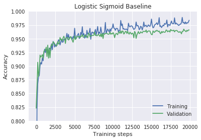
The non-stochastic, non-binary baseline
print("Variance-adjusted:")
res1 = train_classifier(hidden_dims=[100], estimator=StochasticGradientEstimator.REINFORCE, epochs=3,
                       lr=0.3, verbose=True)
Variance-adjusted:
Epoch 0 0.0964
Epoch 1 0.0958
Epoch 2 0.0958
Epoch 3 0.0958
print("Not variance-adjusted:")
res2= train_classifier(hidden_dims=[100], estimator=StochasticGradientEstimator.REINFORCE, epochs=3,
                       lr=0.3, no_var_adj=True, verbose=True)
Not variance-adjusted:
Epoch 0 0.0988
Epoch 1 0.0958
Epoch 2 0.0958
Epoch 3 0.0958
res1 = train_classifier(hidden_dims=[100], estimator=StochasticGradientEstimator.REINFORCE, epochs=20,
                       lr=0.05, label = "Variance-adjusted")
res2= train_classifier(hidden_dims=[100], estimator=StochasticGradientEstimator.REINFORCE, epochs=20,
                       lr=0.05, no_var_adj=True, label = "Not variance-adjusted")

plot_n(res1 + res2, lower_y=0.6, title="Experiment 1: REINFORCE variance adjustment")
Epoch 20 0.9262
Epoch 20 0.9264
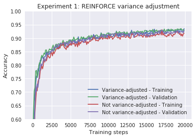
So variance-adjusted learns a bit faster, but it’s not significant.
res1 = train_classifier(hidden_dims=[100], estimator=StochasticGradientEstimator.ST, epochs=20,
                       lr=0.1, label = "Pass-through - 0.1")
res2 = train_classifier(hidden_dims=[100], estimator=StochasticGradientEstimator.ST, epochs=20,
                       lr=0.1, slope_annealing_rate = 1.0, label = "Sigmoid-adjusted - 0.1")

res3 = train_classifier(hidden_dims=[100], estimator=StochasticGradientEstimator.ST, epochs=20,
                       lr=0.3, label = "Pass-through - 0.3")
res4 = train_classifier(hidden_dims=[100], estimator=StochasticGradientEstimator.ST, epochs=20,
                       lr=0.3, slope_annealing_rate = 1.0, label = "Sigmoid-adjusted - 0.3")

res5 = train_classifier(hidden_dims=[100], estimator=StochasticGradientEstimator.ST, epochs=20,
                       lr=1.0, label = "Pass-through - 1.0")
res6 = train_classifier(hidden_dims=[100], estimator=StochasticGradientEstimator.ST, epochs=20,
                       lr=1.0, slope_annealing_rate = 1.0, label = "Sigmoid-adjusted - 1.0")

plot_n(res1[1:] + res2[1:] + res3[1:] + res4[1:] + res5[1:] + res6[1:],
       lower_y=0.4, title="Experiment 2: Pass-through vs sigmoid-adjusted ST")
Epoch 20 0.823
Epoch 20 0.9572
Epoch 20 0.7454
Epoch 20 0.968
Epoch 20 0.0958
Epoch 20 0.9516
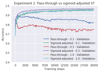
It seems that sigmoid-adjusted beats pass-through by a wide margin
res1 = train_classifier(hidden_dims=[100], estimator=StochasticGradientEstimator.ST, epochs=20,
                       lr=0.1, slope_annealing_rate = 1.0, label = "Sigmoid-adjusted - 0.1")
res2 = train_classifier(hidden_dims=[100], estimator=StochasticGradientEstimator.ST, epochs=20,
                       lr=0.1, slope_annealing_rate = 1.1, label = "Slope-annealed - 0.1")

res3 = train_classifier(hidden_dims=[100], estimator=StochasticGradientEstimator.ST, epochs=20,
                       lr=0.3, slope_annealing_rate = 1.0, label = "Sigmoid-adjusted - 0.3")
res4 = train_classifier(hidden_dims=[100], estimator=StochasticGradientEstimator.ST, epochs=20,
                       lr=0.3, slope_annealing_rate = 1.1, label = "Slope-annealed - 0.3")

res5 = train_classifier(hidden_dims=[100], estimator=StochasticGradientEstimator.ST, epochs=20,
                       lr=1.0, slope_annealing_rate = 1.0, label = "Sigmoid-adjusted - 1.0")
res6 = train_classifier(hidden_dims=[100], estimator=StochasticGradientEstimator.ST, epochs=20,
                       lr=1.0, slope_annealing_rate = 1.1, label = "Slope-annealed - 1.0")

plot_n(res1[1:] + res2[1:] + res3[1:] + res4[1:] + res5[1:] + res6[1:],
       lower_y=0.6, title="Experiment 3: Sigmoid-adjusted vs slope-annealed ST")
Epoch 20 0.9606
Epoch 20 0.9702
Epoch 20 0.9648
Epoch 20 0.9748
Epoch 20 0.9614
Epoch 20 0.9714
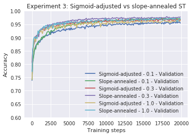
Stochastic sigmoid-adjusted even beats baseline model
res1 = train_classifier(hidden_dims=[100], estimator=StochasticGradientEstimator.ST, epochs=20,
                        lr=0.3, slope_annealing_rate = 1.1, label = "Stochastic, Stochastic")
res2 = train_classifier(hidden_dims=[100], estimator=StochasticGradientEstimator.ST, epochs=20,
                        lr=0.3, slope_annealing_rate = 1.1, stochastic_eval=False, label = "Stochastic, Deterministic")
res3 = train_classifier(hidden_dims=[100], estimator=StochasticGradientEstimator.ST, epochs=20,
                        lr=0.3, slope_annealing_rate = 1.1, stochastic_train=False, stochastic_eval=False,
                        label = "Deterministic, Deterministic")

plot_n(res1 + res2 + res3,
       lower_y=0.6, title="Experiment 5: Stochastic vs Deterministic (Slope-annealed ST)")
Epoch 20 0.9746
Epoch 20 0.9726
Epoch 20 0.9748
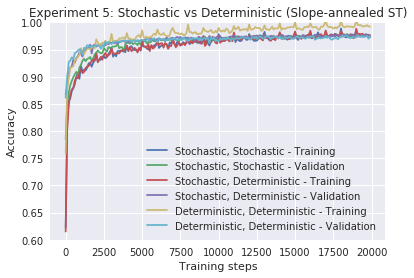
The results show that deterministic neurons train the fastest, but also display more overfitting and may not achieve the best final results. Stochastic inference and deterministic inference, when combined with stochastic training, are closely comparable. Similar results hold for the REINFORCE estimator.
The effect of depth:
It turns out that the slope-annealed straight-through estimator is resilient to depth, even at a reasonable learning rate. The REINFORCE estimator, on the other hand, starts to fail as depth is introduced. However, if we lower the learning rate dramatically (25x), we can start to get the deeper networks to train with the REINFORCE estimator.
res1 = train_classifier(hidden_dims = [200], epochs=20, train_set=mnist.validation, val_set=mnist.test,
                        lr = 0.03, non_binary = True, label = "Deterministic sigmoid net")

res2 = train_classifier(hidden_dims = [200], epochs=20, stochastic_eval=False, train_set=mnist.validation,
                        val_set=mnist.test, slope_annealing_rate=1.1, estimator=StochasticGradientEstimator.ST,
                        lr = 0.3, label = "Binary stochastic net")

plot_n(res1 + res2, lower_y=0.8, title="Experiment 8: Using binary stochastic neurons as a regularizer")
Epoch 20 0.9306
Epoch 20 0.9435

Conclusion:
I skipped some experiments because they don’t seem relevant. Any way in this post, it shows that we can improve upon the performance of an overfitting multi-layer sigmoid net by turning its neurons binary stochastic neurons with a straight-through estimator. And that slope-annealed straight through estimator is better than other straight through variants, and that it is worth using the variance-adjusted REINFORCE estimator over the not variance-adjusted REINFORCE estimator.