A comparison between VAE and GAN

This post concludes VAE and GAN

I’ve took some time going over multiple post regarding VAE and GAN. To help myself to better understand these generative model, I decided to write a post about them, comparing them side by side. Also I want to include the necessary implementation details regarding these two models. For this model, I will use the toy dataset which is MNIST. The code in this post will be mainly implemented with Tensorflow.

VAE

The VAE(variational autoencoder) can be best described as autoencoder with a probability twist.

The motivation behind VAE

The autoencoder is another network architecture that is used to encode object, such as images into latent variables. The latent variables usually have far less dimension and less parameters than the original object. We usually only use the encoder part after we’re finished with the training with autoencoder.

Another use of encoder part of autoencoder is that it can used to initialize a supervised model. Usually fine-tune the encoder jointly with the classifier.

The autoencoder is usually comprised of these module:

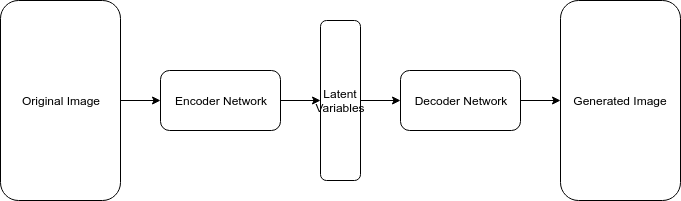
However, simply using the autoencoder to generate images will not be considered as a generative model. Say that you input a image, then the output image you generated will always be the same. In another word, the decoder part of autoencoder network is simply generating things it already remembered.

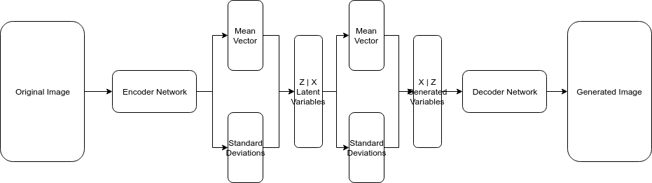
The VAE addresses the above mentioned problem by supplying the latent variables with a sampling technique that makes each feature unit gaussian or some other distribution. In other words, we’ll use the “sampled latent vector” instead of the true latent vector. In the next section will discuss these deductions in detail.

The mathematical proof of VAE

In previous section, we talked about adding a supplementary network to so latent variables can be sampled from it. The mathematical intuition behind this is that alone with the decoder network we cannot calculate the data likelihood. And because of that, the posterior density is also intractable.

Data likelihood:

$$p_\theta(x) = \int p_\theta(z) p_\theta(x | z)dz$$

Posterior density intractable:

$$p_\theta(z | x) = p_\theta(x | z)p_\theta(z)/p_\theta(x)$$

As the integral part of $p_\theta(x)$ is untractable, the posterior density $p_\theta(z | x)$ is also intractable.

Therefore in order to address this issue of intractability, we define additional encoder network $q_\sigma(z | x)$ that approximates $p_\theta(z | x)$.

Now equipped with $q$ the auxillary encoder network, let’s maximize the data likelihood. Please view the full derivation below:

The first two term defines the lower bound on VAE. The third term defines intractable loss. That’s why VAE is optimizing a lower bound on the loss of the likelihood of the data. We can also view the first term $\text{log } p_\theta(x | z)$ as the reconstruction loss. This loss can be estimated via reparametrization trick and L2 binary classification loss. The second term is the KL divergence loss which tries to minimize the difference between posterior distribution $q(z | x)$ and the prior $p(z)$ . We’ll talk about reparametrization trick and KL divergence in the next section.

The reparametrization trick a trick that let us divert the sampling of $p(x | z)$ outside the network. One might ask why not direct sample the $p(x | z)$? This is because directing sampling is a discrete process so it’s not differentiable. In other words, we want to sampling outside the network.

$$\text{Standard Gaussian Distribution: } x_{std} \Longleftarrow x \sim N(\mu, \Sigma)$$ $$\text{Convert to any Gaussian Distribution by shifting and adding: }x = \mu + \Sigma^{\frac{1}{2}} x_{std}$$

The above is the reparametrization trick. We just move the standard Gaussian distribution outside our network. This is best understood with a graph.

The KL divergence loss measures the distance between any two distribution. In our case we want to find out what $D_{KL}[Q(z \vert X) \Vert P(z)]$ is. The $P(z)$ term is easy, it’s just unit Gaussian distribution. Hence we want to make our $Q(z \vert x)$ term as close as possible to $N(0, 1)$, so we that we can sample it easily. Now the KL divergence between two Gaussians do have close-form solution. To save the head-ache I’m just going to spit it out.

$$D_{KL}[N(\mu(X), \Sigma(X)) \Vert N(0, 1)] = \frac{1}{2} \, \left( \textrm{tr}(\Sigma(X)) + \mu(X)^T\mu(X) - k - \log \, \det(\Sigma(X)) \right)$$ $$\text{This can be further reduced to: }$$ $$D_{KL}[N(\mu(X), \Sigma(X)) \Vert N(0, 1)] = \frac{1}{2} \, \sum_k \left( \Sigma(X) + \mu^2(X) - 1 - \log \Sigma(X) \right)$$

Also it’s mentioned in the paper by VAE, that is more numerically stable to take the exponent compared to computing the log, so our formula above can written like this:

$$D_{KL}[N(\mu(X), \Sigma(X)) \Vert N(0, 1)] = \frac{1}{2} \sum_k \left( \exp(\Sigma(X)) + \mu^2(X) - 1 - \Sigma(X) \right)$$

The code for VAE

Once you understand the above math. The code for VAE is exceptionally simple. I will only show the important ones. Those in need can go through the original post at here.

# encoder
def recognition(self, input_images):
    with tf.variable_scope("recognition"):
        h1 = lrelu(conv2d(input_images, 1, 16, "d_h1")) # 28x28x1 -> 14x14x16
        h2 = lrelu(conv2d(h1, 16, 32, "d_h2")) # 14x14x16 -> 7x7x32
        h2_flat = tf.reshape(h2,[self.batchsize, 7*7*32])

        w_mean = dense(h2_flat, 7*7*32, self.n_z, "w_mean")
        w_stddev = dense(h2_flat, 7*7*32, self.n_z, "w_stddev")

    return w_mean, w_stddev

Here in the code, n_z is just the latent variables’ dimension. You can set it to be any number you want. This piece of code simply does convolution followed by standard RELU activation, resulting a 7x7x32 tensor. After that, it reshapes it to a 7x7x32 vector and does fully connected layer from there to output a n_z dimensional vector.

# decoder
def generation(self, z):
    with tf.variable_scope("generation"):
        z_develop = dense(z, self.n_z, 7*7*32, scope='z_matrix')
        z_matrix = tf.nn.relu(tf.reshape(z_develop, [self.batchsize, 7, 7, 32]))
        h1 = tf.nn.relu(conv_transpose(z_matrix, [self.batchsize, 14, 14, 16], "g_h1"))
        h2 = conv_transpose(h1, [self.batchsize, 28, 28, 1], "g_h2")
        h2 = tf.nn.sigmoid(h2) # uses sigmoid instead of softmax, hmm, so this is binary classificiation

    return h2

The decoder part is pretty much the same as the encoder. Except it does transpose convolution. Some people mixes transpose convolution with deconvolution but we will not discuss the difference here. Another thing to notice is that it uses sigmoid instead of softmax for classification, this means it’s a binary classification. There’re some confusion regarding whether we should use this related to our loss function which is L2 loss. But that’s off topic and maybe I’ll write another post about it. For now just assume this is the correct classification to use.

image_matrix = tf.reshape(self.images,[-1, 28, 28, 1])
z_mean, z_stddev = self.recognition(image_matrix)
samples = tf.random_normal([self.batchsize,self.n_z],0,1,dtype=tf.float32)
guessed_z = z_mean + (z_stddev * samples)

self.generated_images = self.generation(guessed_z)
generated_flat = tf.reshape(self.generated_images, [self.batchsize, 28*28])

self.generation_loss = -tf.reduce_sum(self.images * tf.log(1e-8 + generated_flat) + (1-self.images) * tf.log(1e-8 + 1 - generated_flat),1)

self.latent_loss = 0.5 * tf.reduce_sum(tf.square(z_mean) + tf.square(z_stddev) - tf.log(tf.square(z_stddev)) - 1,1)
self.cost = tf.reduce_mean(self.generation_loss + self.latent_loss)
self.optimizer = tf.train.AdamOptimizer(0.001).minimize(self.cost)

The last piece of puzzle is the loss function. This is pretty self-explainatory so I will not say much about it. All we need to focus is the generation_loss and the latent_loss. The generation_loss is just the L2 loss in pixel levels like we talked about at the beginning of the post, while the latent_loss will be the close form solution we got from the last section. Everything else is pretty standard, and Adam trainer and reduce_mean loss overall.

GAN

GAN is another type of network that does generative learning. It be best explained with the game-theory approach.

The motivation behind GAN

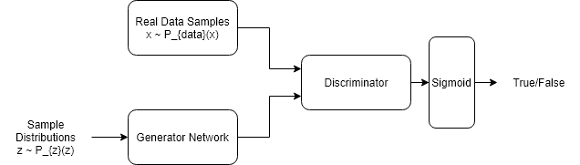
GAN is short for Generative Adversarial Network. As the name suggests, it focuses on the adversarial part of the network. Basically there are two characters in the network. The discriminator and the generator. The generator always tries to forge something to get pass by the discriminator while the discriminator tries its best to distinguish between fake and real samples. As you can see. This is a cat & mouse game. The difficulties in the network is that the discriminator is pretty much always stronger than the generator, therefore it’s necessary to tune the parameters of the network and to balance the generator and the discriminator.

The math behind GAN

The training of the GAN is a fight between the generator and the discriminator. This can be represented mathematically as

$$\min_G\max_DV(D,G)$$ $$V(D,G) = \mathbb{E}_{x \sim p_{data}(x)}[\log D(x)] + \mathbb{E}_{z \sim p_{z}(z)}[\log (1-D(G(z)))]$$

The above equation can then be broken down into two losses in the implementation of GAN. The first part is the $\max_DV(D,G)$ part. This is telling our model to construct the discriminator loss. which is exactly the same equation, but with a negative signs and changing the max objective to a min objective.

$$\max_DV = \min_D-V$$

The second part of the loss is the generator’s loss. Notice that there’s only one G term in the $V(D,G)$ function. $\min_GV(D,G)$ tell us to minimize the V function by alternating the generator. In other words, it tries to minimize the difference between real and fake samples. Since only the second term contribute to the V function. We then rewrite

$$\min_GV = \min_G\mathbb{E}_{z \sim p_{z}(z)}[\log (1-D(G(z)))] = \min_G\mathbb{E}_{z \sim p_{z}(z)}[-\log D(G(z))]$$

So the first loss function optimizes the parameters in the discriminator’s network while the second loss function optimizes the parameters in the generator’s network. The model would take turn turn in training, but we discuss more about it in the next section.

Sampling

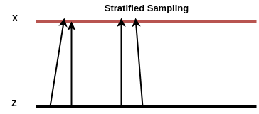
Before we get into the training of GAN, we need to to sample both our data and noise, say for example our data is distributed as $X \sim \mathcal{N}(-1, 1)$ and our noise/latent variable is distributed as $Z \sim \mathcal{N}(0, 1)$. However if we just blindly sample them from two independent resource, the training of GAN will not lead to good result. This is because nothing is enforcing the adjacent pints in the latent space domain being mapped to adjacent points in the X domain (real sample domain). In one minibatch, we might train our generator to map some latent samples to some X domain, however in another minibatch we might points very close to the previous latent samples but mapping to a very different location in X. This implies a completely different mapping G from the previous minibatch, so the optimizer will fail to converge.

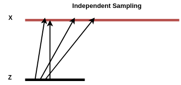
To get over this, we want to use a trick called stratified sampling. That is we want our align our X and Z (latent space) domain so that the total length of the arrows taking points from Z to X is minimized.

Two steps for doing this (for the 1-D example):

1. Stretch the domain of Z to be the same size of X. So that G will not to learn to stretch.
2. Generate $M$ equally spaced points along the domain of Z and then jitter the points randomly. The $M$ stands for the points to sample, both in Z and X.
3. Sort X (Z is already sorted in step 2)

As quoted by Eric Jang in his post regarding GAN:

This step was crucial for me to get this example working: when dealing with random noise as input, failing to align the transformation map properly will give rise to a host of other problems, like massive gradients that kill ReLU units early on, plateaus in the objective function, or performance not scaling with minibatch size.

The code for GAN

The generator part:

def generator(input, hidden_size):
    h0 = tf.nn.softplus(linear(input, hidden_size, 'g0'))
    h1 = linear(h0, 1, 'g1')
    return h1

The generator is simple. It’s linear transformation passed through some non-linear function. Followed by another linear transformation.

The discriminator part:

def discriminator(input, hidden_size):
    h0 = tf.tanh(linear(input, hidden_size * 2, 'd0'))
    h1 = tf.tanh(linear(h0, hidden_size * 2, 'd1'))
    h2 = tf.tanh(linear(h1, hidden_size * 2, 'd2'))
    h3 = tf.sigmoid(linear(h2, 1, 'd3'))
    return h3

The discriminator is more powerful than the generator. Because we want it to be able to learn to distinguish accurately between generated and real samples. It outputs sigmoid in which we can interpret as a probability.

The loss function part:

with tf.variable_scope('G'):
    z = tf.placeholder(tf.float32, shape=(None, 1))
    G = generator(z, hidden_size)

with tf.variable_scope('D') as scope:
    x = tf.placeholder(tf.float32, shape=(None, 1))
    D1 = discriminator(x, hidden_size)
    scope.reuse_variables()
    D2 = discriminator(G, hidden_size)

loss_d = tf.reduce_mean(-tf.log(D1) - tf.log(1 - D2))
loss_g = tf.reduce_mean(-tf.log(D2))

The loss functions, as explained in the mathematical formulation of last section, the goal is to have our generator fool the discriminator. And the discriminator being able to tell the difference between real and generated data.

In order to train model for GAN, we need to draw samples from data distribution and the noise distribution. And alternate between optimizing the parameters of the discriminator and the generator.

with tf.Session() as session:
    tf.initialize_all_variables().run()

    for step in xrange(num_steps):
        # update discriminator
        x = data.sample(batch_size)
        z = gen.sample(batch_size)
        session.run([loss_d, opt_d], {
            x: np.reshape(x, (batch_size, 1)),
            z: np.reshape(z, (batch_size, 1))
        })

        # update generator
        z = gen.sample(batch_size)
        session.run([loss_g, opt_g], {
            z: np.reshape(z, (batch_size, 1))
        })

There are actually many ways to fool the discriminator. In fact if the data generated has a mean value of the real data in this simple example then it is going to be able to fool the discriminator. Collapsing to a parameter setting where it always emits the same point is a common failure mode for GAN.

There are exist many possible solution to this problem. It is not entirely clear how to generalize this to a bigger problem.

Improving the sample diversity

As quoted in the paper “Improved Techniques for Training GANs”:

Because the discriminator processes each example independently, there is no coordination between its gradients, and thus no mechanism to tell the outputs of the generator to become dissimilar to each other.

Therefore it’s easy for the GAN network to collapse to single mode. An technique for elevating this type of failure is obviously let the discriminator make use of the side information when training a batch of samples. This means letting the discriminator look at multiple data examples in combination and perform a so called minibatch discrimination

This is basically doing the following:

• Take the output of the intermediate layer of the discriminator
• Multiply with a 3D tensor to produce a matrix (in code we just multiply 2D matrix then reshape to get 3D tensor, where each sub tensor is of different matrix)
• Compute $L_1$ distance between rows in the this matrix across all samples in a batch
• Apply a negative exponential
• Take the sum of these exponential distances. The result will be [batch_size, kernels]. The “kenerl” is a big aspect of which we want to compared to other samples to
• Concatenate the original input to the minibatch layer and pass to next layer of the discriminator

def minibatch(input, num_kernels=5, kernel_dim=3):
    x = linear(input, num_kernels * kernel_dim)
    activation = tf.reshape(x, (-1, num_kernels, kernel_dim))
    diffs = tf.expand_dims(activation, 3) - \
        tf.expand_dims(tf.transpose(activation, [1, 2, 0]), 0)
    abs_diffs = tf.reduce_sum(tf.abs(diffs), 2)
    minibatch_features = tf.reduce_sum(tf.exp(-abs_diffs), 2)
    return tf.concat(1, [input, minibatch_features])

In Tensorflow it will look like this. The experiment result shows that it makes the generator to maintain most of the width of the original data. Not perfect but much better than plain GAN model.

Comparison and Conclusion

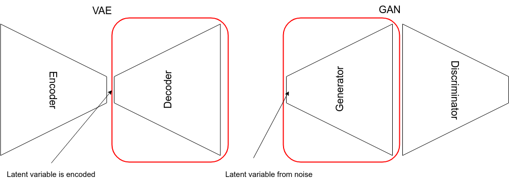
In this post we have gone over two popular generative model. One is the VAE and the other is the GAN. The VAE uses something called density approximation while the GAN use a direct approach that was rooted in game theory. The VAE usually generate a more blurry picture than the GAN. However it does have more control than the plain GAN in terms of what kind of image we want to generate since the latent vector is generated by an encoder whereas in GAN the latent vector comes from random noise. We also see the difference in the loss function as well. The VAN can compare the generated and original samples directly whereas in GAN the generated samples can only be judged fake or real. However the GAN on the other hand generate more realistic images since it make uses of adversarial network. Now this network can be a deep network which would make it more powerful.

One big problem of these generative model is the evaluation of the generated quality. This is still an open area of research and I plan to do some followups on that. It’s also possible to combine VAE and GAN together to fully utilize the best of both to generate certain class of realistic images. This is something we may cover in the future as well.

Reference code

These are some reference code I used to write this post. They are of incredible help.

1-D GAN

VAN MNIST